Training a TensorFlow model for predicting the Genres of Popular Songs
This post is a part of a series where I detail the entire process of making a Genre Classification App using Machine Learning:
- Finding the audios to be classified, i.e. finding the top 50 songs for the last 5 decades (find it here)
- Finding the training data, extracting features from the trendy audios using Librosa (a Python library) (find it here)
- Training the Machine Learning (Tensorflow) model (you’re here!)
- Coming Soon — Creating the Plotly-Dash Application to make a website for the model
- Coming Soon — Deploying the completed app to AWS EC2
The goal
The aim in this post is to detail the process of building a Genre Classification Model in TensorFlow, as well as the different steps in preparing the data to be used in this model. This is quite a lengthy post because I’ve tried to explain as much of the process in detail as possible. Hope this is truly helpful for those interested!
The process
A brief recap
If you’ve seen the last 2 posts, feel free to skip this section as I’ll just be sharing across the basic background.
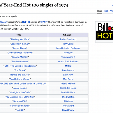
Firstly, I got the top 50 songs from the Billboard Year-End Hot 100 singles for the years 1973–2022. I retrieved this data, and found the YouTube URLs for these songs. Then, from the URLs, I downloaded these songs onto my local machine, to perform further analysis. To check out the step-by-step process for this, please visit the first post in the series.

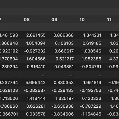
Next, I analysed these audio files using Librosa (Python’s audio library), and extracted the following features: chroma_stft , chroma_cqt, chroma_cens, tonnetz, mfcc, rmse, zcr, spectral_centroid, spectral_bandwidth, spectral_contrast, spectral_rolloff
This the DataFrame that is finally obtained. For the complete process, as well as the code and more information about the above features, please visit the second post in this series.

The model
Perfect, we’re all caught up. The above DataFrame is what we will be running our predictions on, and is created in the exact same way as the training dataset obtained from the mdeff/fma dataset.
Now, we can get to the exciting bit, building the actual TensorFlow model to use all of these features to predict the Genre of our songs.
My artificial intelligence model is a neural network based on deep learning, and it would be best if you had some level of familiarity with the general ideas before jumping into this section. This articles is a wonderful resource on understanding the basics:
Now, since my training data provided me with the genres of the songs, alongside their features, I chose to use Supervised Learning. Supervised Algorithms perform, primarily, two different types of tasks:
- Regression Tasks — These tasks involve predicting a number or a value on a continuous distribution.
- Classification Tasks — This involves, as the name suggests, categorising the input data into one or more of the provided labels.
The task I’m trying to perform is, of course, Genre Classification. This means that my model will try to find the likelihood that any data I input, belongs to one of these labels or classes from my training data, which are: Blues, Classical, Country, Electronic, Experimental, Folk, Hip-Hop, Instrumental, International, Jazz, Old-Time/Historic, Pop, Rock, Spoken.
Now, for setting up the model:
Step 1: Loading and Preprocessing the Data
So, I use Pandas and Scikit-learn (sklearn) here for these tasks.
features = pd.read_csv('/fma-master/data/fma-metadata/features.csv', header=[0,1,2], index_col=0)
tracks = pd.read_csv('/fma-master/data/fma-metadata/tracks.csv', header=[0,1], index_col=0)

tracks = tracks[tracks['track', 'genre_top'].notna()]
tracks = tracks[(tracks['track', 'genre_top'] != "Easy Listening") & (tracks['track', 'genre_top'] != "Soul-RnB")]
The first 2 lines load up the required dataset and the next two lines clean up the dataeset. I drop the data points where the genre is not specified, and where the genres are “Easy Listening” and “Soul-RnB” because there was far too few data points in these genres, and I felt that this was an appropriate bargain to make for increased accuracy.
Next, I used a few columns, and ran a preprocessor on the data. It performs 3 primary functions,
- Encodes all the classes (genres), using sklearn.preprocessing.LabelEncoder, which essentially labels all the classes from 0 to the no_of_classes-1
- Applies the sklearn.preprocessing.StandardScaler, which allows me to scale all my features, and prevents higher or lower value extremes from having a significant influence on the model just by virtue of their numerical values.
- Runs the sklearn.feature_selection.VarianceThreshold, which allows us to remove all features with variance below a certain threshold, and in this, case I used 0.5 as my limit. This prevents features where the data is far too similar for it to have a meaningful impact on the model calculations.
The latter 2 are clubbed together in an sklearn.pipeline.Pipeline construct that allows us to streamline the processes.
The code for implementing the above is, shown here:
columns = ['mfcc', 'spectral_contrast', 'chroma_cens', 'spectral_centroid', 'zcr', 'tonnetz']
features_indexed = features.loc[tracks.index]

def preprocess_2(tracks, features, columns):
  enc = LabelEncoder()
  labels = tracks['track', 'genre_top']
  X = features[columns].sort_index()
  y = tracks['track', 'genre_top'].sort_index()
  X, y = shuffle(X, y, random_state=12)

  X_train, X_test,y_train, y_test = train_test_split(X, y, random_state=42, test_size=0.2)

  y_train = enc.fit_transform(y_train)
  y_test = enc.transform(y_test)

  pipe = Pipeline([
      ('scaler', StandardScaler(copy=False)),
      ('feature_selection', VarianceThreshold(threshold=0.5)),
  ])

  X_train = pipe.fit_transform(X_train, y_train)
  X_test = pipe.transform(X_test)

  return y_train, y_test, X_train, X_test, enc, pipe

y_train, y_test, X_train, X_test, enc, pipe = preprocess_2(tracks, features_indexed, columns)

joblib.dump(pipe, 'pipe.joblib')
joblib.dump(enc, 'enc.joblib')
I save the pipeline and encoder used to ensure that I can transform and perform predictions on any new piece of data, at a later date, using the joblib module.
After the data has been run, I get X_train, X_test, y_train and y_test, with the shapes of these arrays as:
X_train.shape = (39519, 329)
X_test.shape = (9880, 329)
y_train.shape = (39519,)
y_test.shape = (9880,)
This means that I have almost 40000 training data points with 329 features for each of them, and 10000 testing data points.
Step 2: Imbalanced Datasets, and how to deal with them
While exploring the data, I found the number of data points in the training data for each class:
tracks.loc[:, [('track', 'genre_top')]].value_counts()

#And this is the result I obtained
(track, genre_top)
Rock                   14182
Experimental           10608
Electronic              9372
Hip-Hop                 3552
Folk                    2803
Pop                     2332
Instrumental            2079
International           1389
Classical               1230
Jazz                     571
Old-Time / Historic      554
Spoken                   423
Country                  194
Blues                    110
dtype: int64
This is clearly an imbalanced dataset, the number of data points for the top 2 categories are almost 10 times that of the lowest category. This kind of imbalance in the dataset can lead to skewed results in the model, making it biased towards always predicting the classes that are present in a larger number.
This is especially problematic because the model tries to predict everything to be a part of the majority class, and because most of its predictions will be correct, since most of the points do in fact belong to the majority class, it will appear to have a high accuracy, despite making major errors in choosing other classes.
Now, how do we fix this? There are a couple of ways:
- Changing our data, through undersampling or oversampling: Undersampling is using less data from the majority classes, and trying to balance the dataset by reducing the overall number of observations. Oversampling is trying to increase the number of data points in the minority classes, and this is done by extrapolating from the available data points.
- Telling the model to weigh the lower classes more: In a TensorFlow model, the optimizations are made based on how much the error between the actual and predicted labels is, and as I just explained above, the accuracy appears to be high because the model doesn’t consider misclassifying the minority classes as a big problem. So, we tell the model to weigh incorrect predictions against the minority classes more strongly in its calculation of the error, and thus, weigh these classes more.
Both of these options have their pros and cons and after experimenting with the oversampling and undersampling, and class weights technique, I found that the latter worked better for me.
Now there’s a lot of ways to find the weight that should be assigned to the different classes, but it is generally a variation on max_count/class_count , this would make the weights of all classes ≥1. With a little experimentation I found that for my case, this was the formula that worked best.
classes, counts = np.unique(y_train, return_counts=True)
max_count = counts.max()
weights = {}

for i in range(len(counts)):
  count = counts[i]
  weights[i] = math.ceil(max_count/(count)+1) #the +1 creates a buffer in the weights
Alright, now that we’ve figured out a way to deal with the imbalance in the dataset, let’s get into the model.
Step 3: The TensorFlow Model FINALLY!
Alright, so hoping that you have a basic understanding of AI, let’s finally discuss the model.
With a lot of experimentation, this was the model architecture I found to have the best performance. I did start off with a normal ANN architecture, but my data was structured in a way that gave me the idea that I could use a Convolutional Architecture.
Convolutional layers consist of filters, which are used to detect improtant patterns. These are normally used for images, and is used to identify curves or textures. These filters lead to a lot of data being produced, as these filters perform multiple ocmplex operations over all the available data. After the ConvLayer, Pooling layers are added to help reduce the amount of data that has to be dealt with, while keeping the essential information intact.
To learn more about the Convolutional Neural Network, check out https://towardsdatascience.com/covolutional-neural-network-cb0883dd6529

Now, while I don’t have images, which normally use a 2D Convolutional Network, I could instead use the 1-Dimensional Filter Layer.
My CNN has multiple layers of filters, and they learn by adjusting the filter parameters during training to recognize complex features. Multiple layers of the convolution, also allows for hierarchical feature extraction. This is the structure that gave me the best results:
model = tf.keras.Sequential()
model.add(Input(shape=(X_train.shape[1])))
model.add(Reshape((X_train.shape[1], 1)))
model.add(Conv1D(128, 12, activation='relu')) #mod_4 had 128 mod_5 had 64
model.add(MaxPooling1D())
model.add(Conv1D(64, 12, activation='relu'))
model.add(Flatten())
model.add(Dense(512, activation='relu'))
model.add(Dropout(0.5))
model.add(Dense(64, activation='relu'))
model.add(Dense(32, activation='relu'))
model.add(Dense(len(np.unique(y_train)), activation='softmax'))
For a little more context:
- tf.keras.Sequential, which is used to initialise the model is basically a paradigm that allows you to add layers into the model in a sequential manner.
- The following are all part of the tf.keras.layers submodule:
- the Input layer is defined with the input_shape expected being obtained from the X_train shape, so that it can interpret the number of features in the data point
- the Reshape layer is required to make sure that my data can be used in the Convolutional layer next
- the Conv1D and MaxPooling1D basically perform the functions for convolution as I explained above.
- the Flatten layer, in effect, undoes the effect of the Reshape layer and allows the flattened data to be used in regular Dense layers
- the Dense layers, are layers with a given number of units, and in this layer, we have all the units connected to each other, and the weights can be changed.
- the Dropout layer, essentially disables a few of the weights that makes the model more efficient and lighter (PS: this is not nearly a complete explanation)
And now, we just set up the specific settings, such as the optimisers, losses and hyperparameters and we’re ready to go! The code for the same is:
adam = tf.keras.optimizers.Adam(learning_rate=0.001)
model.compile(loss=tf.keras.losses.SparseCategoricalCrossentropy(),
              optimizer=adam)
There are two things worth explaining here, the optimizer Adam and the loss Sparse Categorical Cross Entropy. The loss essentially signifies the cost or error between the accurate label and the predicted label. The reason for choosing this specific loss is because my labels are one-hot encoded categories. Now one we’ve calculated the loss, we use the optimizer, in this case, Adam, to figure out how the model needs to change to reduce the losses.
For more on Optimizers and Adam: https://towardsdatascience.com/optimizers-for-training-neural-network-59450d71caf6
For more on losses: https://towardsdatascience.com/what-is-loss-function-1e2605aeb904
Now, to reiterate, the choice of optimizers, the values for the hyperparameters, and the architecture of the model are a result of extensive experimentation, and work differently for different use-cases for AI models.
Alright then, just one last step now, let’s run the model!
es_callback = keras.callbacks.EarlyStopping(monitor='val_loss', patience=5)
checkpoint = ModelCheckpoint(filepath,monitor='val_loss',mode='min',save_best_only=True)

history = model.fit(X_train, y_train,
                    class_weight=weights,
                    validation_split = 0.1,
                    batch_size=2048,
                    epochs=100, verbose=1,
                    callbacks=[es_callback, checkpoint])
The model is fitted with the data we have, using an EarlyStopping and ModelCheckpoint as measures to improve the recording and accuracy of the model. Check out the links to learn more about them.
Now, here we use the X_train and y_train datasets that we’ve created along with the weights created to counter the imbalance in the dataset. The batch_size here is rather high that makes the training resource-intensive and time-consuming, but it’s well worth the wait. The epochs signifies the number of times the model should train, and the verbose argument being set to 1 ensures I can see the progress as the model is trained.
We can see the progress in training as:
plt.plot(history.history['loss'])
plt.plot(history.history['val_loss'])
In my graph the training loss remains higher than the validation loss, but they are both consistently reducing. The reason for this difference is because of the way my data is structured, and the imbalance I was dealing with.
Step 4: Checking the model
As I mentioned in the section on imbalanced dataset, it is often difficult to debug the accuracy of the model on such datasets, but there are metrics such as the ROC_AUC_Score that is considered a fairly good bechmark for balanced and imbalanced data alike.
Learn more about the metric at:
https://towardsdatascience.com/imbalanced-data-stop-using-roc-auc-and-use-auprc-instead-46af4910a494
To implement it, I had to first run my model on the test dataset to get predictions, and convert it into a usable format for the metric using the sklearn.preprocessing.LabelBinarizer.
preds_test = model.predict(X_test)
preds_test = np.argmax(preds_test, axis=1)

from sklearn.preprocessing import LabelBinarizer

label_binarizer = LabelBinarizer().fit(y_train)
y_onehot_test = label_binarizer.transform(y_test)
preds_onehot_test = label_binarizer.transform(preds_test)
Now, to run the metric, there are two options to run it that I considered, the average=None provides a list of the roc_auc_score for each class in a list, and the average='weighted' provides the average of all the scores weighted by their class number.
print(roc_auc_score(y_onehot_test, preds_onehot_test, average=None))
print(roc_auc_score(y_onehot_test, preds_onehot_test, average='weighted'))
#and this is the result that I obtained:
[0.72444219 0.88212985 0.79329675 0.79628912 0.78339301 0.82810634
0.86196564 0.69422879 0.78670436 0.76173557 0.98794697 0.64119238
0.85371012 0.85083461]
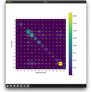
0.808511463879435In this particular run, I got a 0.782 weighted accuracy, with eatleast 70% accuracy for all but one of the classes. Analysing the exact distribution of the classes can be done using a Confusion Matrix:
from sklearn.metrics import confusion_matrix, ConfusionMatrixDisplay
cm = confusion_matrix(y_test, preds_test)
disp = ConfusionMatrixDisplay(confusion_matrix=cm)
fig, ax = plt.subplots(figsize=(8,8))
disp.plot(ax=ax)
A Confusion Matrix essentially shows the number of predictions with the true_label mapped against the predicted_label for each class. Ideally, the primary diagonal should be the brightest, which does show up in this diagram, however, for some classes, the accuracy still remains poor. It is important to note that because the data is imbalanced, the colors do not quite show strongly on the diagonal, but it is easy to check that the value on the diagonal is the highest for all the predictions for any label. This is the result we get:

While this was the latest iteration of my model, it wasn’t the best, however I ensured version control, and maintained a record of the one’s with the best accuracy. I would do this by saving the trained model, and mapping it to its metrics.
So, once we’re done with the final training and we’re comfortable with our model, let’s save this model in a h5py file: model.save('model.h5')
And that’s it! We’ve created a TensorFlow model, and we’ve measured it’s accuracy, and saved it for future use!
The Debugging
Alright, I know that this post ahs already grown quite large, but I still have a few important points to make about all of the things I’ve discussed on this post:
- Be sure to explore your data in as many different ways as possible. It is critical that you know what problems may arise if your data is of certain types, like dealing with an imbalanced dataset in my example.
- Be ready to experiment with the different ways of solving your problems. The reason I shared the under- and over-sampling techniques despite not using them in my final run is because it was a step that I took, and then I had to entirely drop the idea, after experimenting with just undersampling or oversampling or a combination of both. It is important that we try and make mistake and find the answer that suits us best.
- Be willing to try a new paradigm — if I had remained stuck to the resular dense ANN structure, I would not have been able to reach the accuracy I have now.
- Try out different options— there are a lot of variables to change.
- For example, in the preprocessing, I could tweak the
variancein the feature_selection that I performed with VarianceThreshold, or I could use an entirely different technique, and I did — I tried using a function called SelectKBest, which tries to selectkbest predictors for the label, again, here I tweaked the value ofkmultiple times. - The optimizer I used is Adam, but I also experimented with simple Stochastic Gradient Descent. Again, in the Adam optimizer, the
learning_ratewas an important parameter in the performance of the model. - The weights for the classes were found out of atleast a hundred of the different variations I had created while mapping and comparing the performance with regards to each of the classes using the Confusion Matrix.
- And finally, the model is never right in the first go, or even on the 10th try. Keep trying and pushing the architecture, but understand what errors could be occuring and learn how to solve them. A simple example would be if your training loss while plotting is getting smaller while your validation loss in training stagnates, you might be overfitting the model.

That’s all I have for you all now! Next time, I’ll be explaining a few caveats with the interprettation of the results of my model and will be using this model to run predictions on my collected data and show you how to create a Dashboard using Plotly to show this data and share the model on your website!
Visit the complete list of stories for this project at:
The code with the data and how to collect it, along with the code for the model is available at: